We have various kinds of the software for creating graph. ''Gnuplot'' is the one which has a much broader range of applications since it can draw the graph from not only the data, but also functions. Furthermore, you can apply the fitting the data, draw the 3D graph etc.,
while the programming needs to be done.
Numerical differentiation & integration can also be easily indicated as you become familiar. Furthermore, even though the differential equation is very complicated, the graph of the numerical solution can be drawn once the programming is completed. One of the advantages of the ''Gnuplot'' is that the numerical analysis can be simultaneously done on the creating graph program.
The numerical analysis of the differential equation can be generally done by the following algorithm. Firstly, based on the definition of the differentiation, the equation (1) can be proven.
\begin{eqnarray}
y'=f(x,y)=\lim_{h \to 0} \frac{y(x+h)-y(x)}{h}
\end{eqnarray}
When ''$h$'' is small, it becomes the equation (2).
\begin{eqnarray}
f(x,y)\approx \frac{y(x+h)-y(x)}{h} \nonumber \\
y(x+h)\approx y(x)+hf(x,y)
\end{eqnarray}
Assuming that the default values of ''$x$'' & ''$y$'' are ''$x_0$'' & ''$y_0$'' respectively, and assuming that the equations ''$x_1$'' & ''$y_1$'' are as follows, ''$x_{n+1}$'' & ''$y_{n+1}$'' can be indicated as shown in the equations (3) & (4) respectively.
\begin{eqnarray}
x_1&=&x_0+h,x_2=x_1+h,\cdots \nonumber \\
y_1&=&y_0+hf(x_0,y_0),y_2=y_1+hf(x_1.y_1),\cdots \nonumber
\end{eqnarray}
\begin{eqnarray}
x_{n+1}&=&x_n+h \\
y_{n+1}&=&y_n+hf(x_n,y_n)
\end{eqnarray}
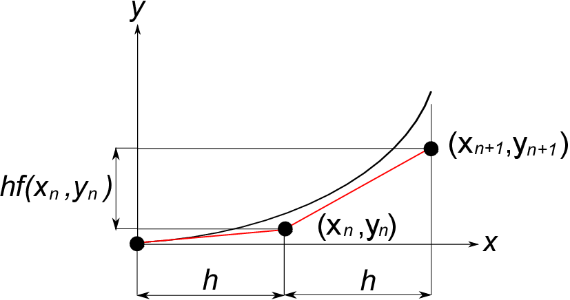
In the numerical analysis, calculating this repeatedly on the computer, the whole shape of the function ''$y$'' is approximated. This is known as Euler's method as shown in the figure below.

From this chart, when ''$x$'' is increased by ''$h$'', the increment of ''$y$'' is ''$hf (x_n, y_n)$''. Accordingly, ''$f(x_n,y_n)$'' indicates the local gradient of the function ''$y$''. In order to predict ''$y_{n+1}$'' from ''$x_n$'' & ''$y_n$'', it is important to precisely obtain this local gradient. For example, what the accuracy of the approximation is improved based on ''$\frac{1}{2}[f(x_n,y_n)+f(x_{n+1},y_n+hf(x_n,y_n))]$'' for gradient ''$f(x_n,y_n)$'' is known as Heun's method.
In terms of the Runge-Kutta method (RK4), sorting the gradient into four kinds, and applying the weighting for these further, it is defined as shown in the equation (5).
\begin{eqnarray}
y'&=&f(x,y), \;\;\;y(x_0)=y_0 \nonumber \\
y_{n+1}&=&y_n+\frac{h}{6}(k_1+2k_2+2k_3+k_4) \nonumber \\
k_1&=&f(x_n,y_n) \nonumber \\
k_2&=&f(x_n+\frac{h}{2},y_n+\frac{h}{2}k_1) \nonumber \\
k_3&=&f(x_n+\frac{h}{2},y_n+\frac{h}{2}k_2) \nonumber \\
k_4&=&f(x_n+h,y_n+hk_3)
\end{eqnarray}
In view of the accuracy and the calculation time relationship, the Runge-Kutta method (RK4) is superior to other ones, while there are various kinds of the numerical solutions in figuring out the differential equation.
The calculation accuracy is approx. fourth power of the increment, ''$h$''. For example, if the increment, ''$h$'' is ''$10^{-2}$'', the accuracy will be approx. ''$10^{-8}$''.
Then, we apply the Runge-Kutta method (RK4) by taking the example of the equation of motion of the pendulum which is shown in the equation (6) below.
\begin{eqnarray}
ml\frac{d^2\theta}{dt^2}=-mgsin\theta
\end{eqnarray}
In the Section 1, the assumption of ''$sin\theta\approx\theta$'' was applied in order to obtain the approximate theoretical solution. However, it is not necessary in case of the numerical analysis.
Dividing the both sides of the equation (6) by ''$ml$'', the equation (7) can be obtained.
\begin{eqnarray}
\frac{d^2\theta}{dt^2}=-\frac{g}{l}sin\theta
\end{eqnarray}
As this is a second order differential equation, it needs to be converted to the simultaneous first order differential equations as shown in the following so that the Runge-Kutta method (RK4) can be leveraged.
\begin{eqnarray}
\frac{d\omega}{dt}&=&-\frac{g}{l}sin\theta \\
\frac{d\theta}{dt}&=&\omega
\end{eqnarray}
As for the rest, all you have to do is sequentially calculate the factors in accordance with the equation (5), and obtain ''$\theta_{n+1},\omega_{n+1}$''. Be noted that the functions need to be separated to ''$f(t,\theta,\omega)$'' and '' $g(t,\theta,\omega)$'' in addition to the use of ''$k$'' & ''$m$'' for the factors, simply because of the simultaneous differential equation in this case.
You do not have to take it complicated in terms of the simultaneous equation, but it can be, so to speak, automatically solved by calculating such factors equations as shown in the following in the simultaneous and parallel manner.
The below indicates how to calculate.
\begin{eqnarray}
&\;&f(\theta,\omega,t)=\frac{d\omega}{dt}=-\frac{g}{l}sin\theta \nonumber \\
&\;&g(\theta,\omega,t)=\frac{d\theta}{dt}=\omega \nonumber \\
\end{eqnarray}
\begin{eqnarray}
&k_1&=f(\theta_n,\omega_n,t_n) \nonumber \\
&m_1&=g(\theta_n,\omega_n,t_n) \nonumber \\
&k_2&=f(\theta_n+0.5m_1,\omega_n+0.5k_1,t_n+0.5h) \nonumber \\
&m_2&=g(\theta_n+0.5m_1,\omega_n+0.5k_1,t_n+0.5h) \nonumber \\
&k_3&=f(\theta_n+0.5m_2,\omega_n+0.5k_2,t_n+0.5h) \nonumber \\
&m_3&=g(\theta_n+0.5m_2,\omega_n+0.5k_2,t_n+0.5h) \nonumber \\
&k_4&=f(\theta_n+m_3,\omega_n+k_3,t_n+h) \nonumber \\
&m_4&=g(\theta_n+m_3,\omega_n+k_3,t_n+h) \nonumber
\end{eqnarray}
\begin{eqnarray}
&\theta_{n+1}&=\theta_n+\frac{h}{6}(k_1+2k_2+2k_3+k_4) \nonumber \\
&\omega_{n+1}&=\omega_n+\frac{h}{6}(m_1+2m_2+2m_3+m_4) \nonumber
\end{eqnarray}
As shown in the above, all you need is to describe the program like the above, and to sequentially calculate these equations. The sample programs for some selected primary subjects in which many readers are also interested are included in the next clause 4-2 for your reference.